Introduction
This vignette demonstrates how to use the hmetad package
to fit the meta-d’ model (Maniscalco & Lau, 2012) to a
canonical metacognition experiment which requires a binary decision
together with a confidence rating on each trial.
Data preparation
To get a better idea of what kind of datasets the hmetad
package is designed for, we can start by simulating one (see
help('sim_metad') for a description of the data simulation
function):
library(tidyverse)
library(tidybayes)
library(hmetad)

d <- sim_metad(
  N_trials = 1000, dprime = .75, c = -.5, log_M = -1,
  c2_0 = c(.25, .75, 1), c2_1 = c(.5, 1, 1.25)
)
#> # A tibble: 1,000 × 4
#> # Groups: stimulus, response, confidence [16]
#> trial stimulus response confidence
#> <int> <int> <int> <int>
#> 1 1 0 0 1
#> 2 2 0 0 1
#> 3 3 0 0 1
#> 4 4 0 0 1
#> 5 5 0 0 1
#> 6 6 0 0 1
#> 7 7 0 0 1
#> 8 8 0 0 1
#> 9 9 0 0 1
#> 10 10 0 0 1
#> # ℹ 990 more rowsAs you can see, our dataset has a column for the trial
number, the presented stimulus on each trial
(0 or 1), the participant’s type 1 response
(0 or 1), and the corresponding type 2
response (confidence; 1:K). The trials in this dataset are
sorted by stimulus, response, and
confidence because this data set is simulated, but
otherwise this should look very similar to the kind of data that you
would get from running your own experiment.
Type 1, type 2, and joint responses
One wrinkle is that some paradigms do not collect a separate decision
(i.e., type 1 response) and confidence rating (i.e., type 2
response)—rather, they collect a single rating reflecting both the
primary decision and confidence. For example, instead of a binary type 1
response and a type 2 response ranging from 1 to
K (where K is the maximum confidence level),
sometimes participants are asked to make a rating on a scale from
1 to 2*K, where 1 represents a
confidence "0" response, K represents an
uncertain "0" response, K+1 represents an
uncertain "1" response, and 2*K represents a
confident "1" response. We will refer to this as a
joint response, as it is a combination of the type 1 response
and the type 2 response.
If you would like to convert joint response data into separate type 1
and type 2 responses, you can use the corresponding functions
type1_response and type2_response. For
example, if instead we had a dataset that looked like this:
#> # A tibble: 1,000 × 2
#>    trial joint_response
#>    <int>          <int>
#>  1     1              4
#>  2     2              4
#>  3     3              4
#>  4     4              4
#>  5     5              4
#>  6     6              4
#>  7     7              4
#>  8     8              4
#>  9     9              4
#> 10    10              4
#> # ℹ 990 more rows
Then we could convert our joint response like so:
d.joint_response |>
  mutate(
    response = type1_response(joint_response, K = 4),
    confidence = type2_response(joint_response, K = 4)
  )
#> # A tibble: 1,000 × 4
#>    trial joint_response response confidence
#>    <int>          <int>    <int>      <dbl>
#>  1     1              4        0          1
#>  2     2              4        0          1
#>  3     3              4        0          1
#>  4     4              4        0          1
#>  5     5              4        0          1
#>  6     6              4        0          1
#>  7     7              4        0          1
#>  8     8              4        0          1
#>  9     9              4        0          1
#> 10    10              4        0          1
#> # ℹ 990 more rows
Similarly, you can also convert the separate responses into a joint response:
d |>
  mutate(joint_response = joint_response(response, confidence, K = 4))
#> # A tibble: 1,000 × 5
#> # Groups:   stimulus, response, confidence [16]
#>    trial stimulus response confidence joint_response
#>    <int>    <int>    <int>      <int>          <int>
#>  1     1        0        0          1              4
#>  2     2        0        0          1              4
#>  3     3        0        0          1              4
#>  4     4        0        0          1              4
#>  5     5        0        0          1              4
#>  6     6        0        0          1              4
#>  7     7        0        0          1              4
#>  8     8        0        0          1              4
#>  9     9        0        0          1              4
#> 10    10        0        0          1              4
#> # ℹ 990 more rows
Note that in both cases we need to specify that our confidence scale
has K=4 levels (meaning that our joint type 1/type 2 scale
has 8 levels).
Signed and unsigned binary numbers
Often datasets will use -1 and 1 instead of
0 and 1 to represent the two possible stimuli
and type 1 responses. While the hmetad package is designed
to use the unsigned (0 or 1) version,
it provides helper functions to convert between the two:
to_unsigned(c(-1, 1))
#> [1] 0 1Data aggregation
Finally, to ensure that the model runs efficiently, the
hmetad package currently requires data to be aggregated. If
it is easier, the hmetad package will aggregate your data
for you when you fit your model. But if you would like to do so manually
(e.g., for plotting or follow-up analyses), the
aggregate_metad function can do this for you:
d.summary <- aggregate_metad(d)
#> `hmetad` has inferred that there are K=4 confidence levels in the data. If this is incorrect, please set this manually using the argument `K=<K>`
#> # A tibble: 1 × 3
#> N_0 N_1 N[,"N_0_1"] [,"N_0_2"] [,"N_0_3"] [,"N_0_4"] [,"N_0_5"] [,"N_0_6"]
#> <int> <int> <int> <int> <int> <int> <int> <int>
#> 1 500 500 3 59 117 44 83 135
#> # ℹ 1 more variable: N[7:16] <int>The resulting data frame has three columns: N_0 is the
number of trials with stimulus==0, N_1 is the
number of trials with stimulus==1, and N is a
matrix containing the number of joint responses for each of the two
possible stimuli (with column names indicating the stimulus
and joint_response).
If you would like to use variable name other than N for
the counts, you can change the name with the .name
argument:
aggregate_metad(d, .name = "y")
#> `hmetad` has inferred that there are K=4 confidence levels in the data. If this is incorrect, please set this manually using the argument `K=<K>`
#> # A tibble: 1 × 3
#> y_0 y_1 y[,"y_0_1"] [,"y_0_2"] [,"y_0_3"] [,"y_0_4"] [,"y_0_5"] [,"y_0_6"]
#> <int> <int> <int> <int> <int> <int> <int> <int>
#> 1 500 500 3 59 117 44 83 135
#> # ℹ 1 more variable: y[7:16] <int>Similarly, you are able to use different column names for
stimulus, response, and
confidence (or stimulus and
joint_response):
d |>
rename(
s = stimulus,
r = response,
c = confidence
) |>
aggregate_metad(.stimulus = "s", .response = "r", .confidence = "c")
#> `hmetad` has inferred that there are K=4 confidence levels in the data. If this is incorrect, please set this manually using the argument `K=<K>`
#> # A tibble: 1 × 3
#>     N_0   N_1 N[,"N_0_1"] [,"N_0_2"] [,"N_0_3"] [,"N_0_4"] [,"N_0_5"] [,"N_0_6"]
#>   <int> <int>       <int>      <int>      <int>      <int>      <int>      <int>
#> 1   500   500           3         59        117         44         83        135
#> # ℹ 1 more variable: N[7:16] <int>If you have other columns in your dataset (e.g.,
participant or condition columns) that you
would like to be aggregated separately, you can simply add them to the
function call:
aggregate_metad(d, participant, condition)Finally, note that aggregate_metad automatically
estimates the number of confidence levels based on the maximum value of
the confidence or joint response column in your data. This usually works
fine, but may fail in cases with missing data (e.g., no participant
gives a confidence rating of 3 on a 4-point
scale). The number of confidence levels can be specified manually using
the argument K:
aggregate_metad(d, participant, condition, K = 4)Model fitting
To fit the model, we can use the fit_metad function.
This function is simply a wrapper around brms::brm, so
users are strongly encouraged to become familiar with
the brms
package before model fitting. In particular, users are likely to run
into convergence errors using the default (flat) priors for model
parameters, so we recommend doing careful prior predictive checks to set
weakly informed priors (see Schad et al., 2021 for more
information).
Since aggregate_metad will place our dataset has our
trial counts into a column named N by default, we can use
N as our response variable even if our data is not yet
aggregated. To fit a model with fixed values for each parameter, then,
we can use the formula N ~ 1:
m <- fit_metad(N ~ 1,
  data = d, init = 0,
  prior = prior(normal(0, 1), class = Intercept) +
    prior(normal(0, 1), class = dprime) +
    prior(normal(0, 1), class = c) +
    set_prior("lognormal(0, 1)", class = metac2_parameters(K = 4))
)
#> Family: metad__4__normal__absolute__multinomial
#> Links: mu = log
#> Formula: N ~ 1
#> Data: data.aggregated (Number of observations: 1)
#> Draws: 4 chains, each with iter = 2000; warmup = 1000; thin = 1;
#> total post-warmup draws = 4000
#>
#> Regression Coefficients:
#> Estimate Est.Error l-95% CI u-95% CI Rhat Bulk_ESS Tail_ESS
#> Intercept -0.69 0.33 -1.43 -0.12 1.00 4446 2542
#>
#> Further Distributional Parameters:
#> Estimate Est.Error l-95% CI u-95% CI Rhat Bulk_ESS Tail_ESS
#> dprime 0.71 0.09 0.54 0.88 1.00 6394 3014
#> c -0.49 0.04 -0.58 -0.41 1.00 4587 3335
#> metac2zero1diff 0.21 0.02 0.17 0.26 1.00 6569 2623
#> metac2zero2diff 0.78 0.06 0.68 0.90 1.00 6385 3291
#> metac2zero3diff 1.25 0.17 0.94 1.61 1.01 7202 2919
#> metac2one1diff 0.47 0.03 0.41 0.54 1.00 5110 3275
#> metac2one2diff 1.00 0.05 0.91 1.09 1.00 6801 3074
#> metac2one3diff 1.29 0.11 1.09 1.51 1.00 6541 3022
#>
#> Draws were sampled using sampling(NUTS). For each parameter, Bulk_ESS
#> and Tail_ESS are effective sample size measures, and Rhat is the potential
#> scale reduction factor on split chains (at convergence, Rhat = 1).Note that here we have arbitrarily chosen to use standard normal
priors for all parameters. To get a better idea of how to set informed
priors, please refer to
help('set_prior', package='brms').
In this model, Intercept is our estimate of \textrm{log}(M) =
\textrm{log}\frac{\textrm{meta-}d'}{d'},
dprime is our estimate of d', c is our estimate of
c, metac2zero1diff and
metac2zero2diff are the distances between successive
confidence thresholds for "0" responses, and
metac2one1diff and metac2one2diff are the
distances between successive confidence thresholds for "1"
responses. For each parameter, brms shows you the posterior
means (Estimate), posterior standard deviations
(Est. Error), upper- and lower-95% posterior quantiles
(l-95% CI and u-95% CI), as well as some
convergence metrics (Rhat, Bulk_ESS, and
Tail_ESS).
Manual model fitting
Most users can use fit_metad as above to fit their
models. But in some cases, it might be preferable to call
brms::brm directly. In such cases, the
fit_metad function is roughly analogous to the following
code:
# calculate number of confidence levels
K <- n_distinct(d$confidence)

m <- brm(bf(...),
  data = aggregate_metad(d, ...),
  family = metad(K = K, ...),
  stanvars = stanvars_metad(K = K, ...),
  ...
)
Alternatively, if the only issue is with the automatic data
aggregation, one can provide the argument aggregate=FALSE
to fit_metad:
d.aggregated <- aggregate_metad(d, ...)

# modify d.aggregated as needed

m <- fit_metad(bf(...), d.aggregated, aggregate = FALSE)
Extract model estimates
Once we have our fitted model, there are many estimates that we can
extract from it. Although brms provides its own functions
for extracting posterior estimates, the hmetad package is
designed to interface well with the tidybayes package to
make it easier to work with model posterior samples.
Parameter estimates
First, it is often useful to extract the posterior draws of the model
parameters, which we can do with linpred_draws_metad (which
is a wrapper around tidybayes::linpred_draws):
draws.metad <- tibble(.row = 1) |>
  add_linpred_draws_metad(m)
#> # A tibble: 4,000 × 15
#> # Groups: .row [1]
#> .row .chain .iteration .draw M dprime c meta_dprime meta_c
#> <int> <int> <int> <int> <dbl> <dbl> <dbl> <dbl> <dbl>
#> 1 1 NA NA 1 0.419 0.846 -0.536 0.355 -0.536
#> 2 1 NA NA 2 0.650 0.625 -0.534 0.406 -0.534
#> 3 1 NA NA 3 0.425 0.817 -0.480 0.347 -0.480
#> 4 1 NA NA 4 0.652 0.611 -0.437 0.398 -0.437
#> 5 1 NA NA 5 0.622 0.555 -0.494 0.345 -0.494
#> 6 1 NA NA 6 0.655 0.654 -0.520 0.428 -0.520
#> 7 1 NA NA 7 0.679 0.660 -0.493 0.448 -0.493
#> 8 1 NA NA 8 0.656 0.711 -0.497 0.467 -0.497
#> 9 1 NA NA 9 0.599 0.796 -0.426 0.477 -0.426
#> 10 1 NA NA 10 0.175 0.557 -0.550 0.0973 -0.550
#> # ℹ 3,990 more rows
#> # ℹ 6 more variables: meta_c2_0_1 <dbl>, meta_c2_0_2 <dbl>, meta_c2_0_3 <dbl>,
#> # meta_c2_1_1 <dbl>, meta_c2_1_2 <dbl>, meta_c2_1_3 <dbl>This tibble has a separate row for every posterior
sample and a separate column for every model parameter. This format is
useful for some purposes, but it will often be useful to pivot it so
that we have a separate row for each model parameter and posterior
sample:
draws.metad <- tibble(.row = 1) |>
  add_linpred_draws_metad(m, pivot_longer = TRUE)
#> # A tibble: 44,000 × 6
#> # Groups: .row, .variable [11]
#> .row .chain .iteration .draw .variable .value
#> <int> <int> <int> <int> <chr> <dbl>
#> 1 1 NA NA 1 M 0.419
#> 2 1 NA NA 1 dprime 0.846
#> 3 1 NA NA 1 c -0.536
#> 4 1 NA NA 1 meta_dprime 0.355
#> 5 1 NA NA 1 meta_c -0.536
#> 6 1 NA NA 1 meta_c2_0_1 -0.748
#> 7 1 NA NA 1 meta_c2_0_2 -1.53
#> 8 1 NA NA 1 meta_c2_0_3 -2.97
#> 9 1 NA NA 1 meta_c2_1_1 -0.125
#> 10 1 NA NA 1 meta_c2_1_2 0.937
#> # ℹ 43,990 more rowsNow that all of the posterior samples are stored in a single column
.value, it is easy to get posterior summaries using
e.g. tidybayes::median_qi:
draws.metad |>
  median_qi()
#> # A tibble: 11 × 8
#>     .row .variable    .value .lower  .upper .width .point .interval
#>    <int> <chr>         <dbl>  <dbl>   <dbl>  <dbl> <chr>  <chr>
#>  1     1 c           -0.492  -0.579 -0.406    0.95 median qi
#>  2     1 dprime       0.707   0.545  0.878    0.95 median qi
#>  3     1 M            0.519   0.239  0.885    0.95 median qi
#>  4     1 meta_c      -0.492  -0.579 -0.406    0.95 median qi
#>  5     1 meta_c2_0_1 -0.706  -0.794 -0.616    0.95 median qi
#>  6     1 meta_c2_0_2 -1.49   -1.61  -1.37     0.95 median qi
#>  7     1 meta_c2_0_3 -2.72   -3.11  -2.42     0.95 median qi
#>  8     1 meta_c2_1_1 -0.0195 -0.102  0.0587   0.95 median qi
#>  9     1 meta_c2_1_2  0.978   0.884  1.07     0.95 median qi
#> 10     1 meta_c2_1_3  2.27    2.06   2.49     0.95 median qi
#> 11     1 meta_dprime  0.369   0.171  0.578    0.95 median qi
Posterior predictions
One way to evaluate model fit is to perform a posterior
predictive check: to simulate data from the model’s posterior and
compare our simulated and actual data. We can do this using the function
predicted_draws_metad (which is a wrapper around
tidybayes::predicted_draws):
draws.predicted <- predicted_draws_metad(m, d.summary)#> # A tibble: 64,000 × 12
#> # Groups: .row, N_0, N_1, N, stimulus, joint_response, response, confidence
#> # [16]
#> .row N_0 N_1 N[,"N_0_1"] stimulus joint_response response confidence
#> <int> <int> <int> <int> <int> <int> <int> <dbl>
#> 1 1 500 500 3 0 1 0 4
#> 2 1 500 500 3 0 1 0 4
#> 3 1 500 500 3 0 1 0 4
#> 4 1 500 500 3 0 1 0 4
#> 5 1 500 500 3 0 1 0 4
#> 6 1 500 500 3 0 1 0 4
#> 7 1 500 500 3 0 1 0 4
#> 8 1 500 500 3 0 1 0 4
#> 9 1 500 500 3 0 1 0 4
#> 10 1 500 500 3 0 1 0 4
#> # ℹ 63,990 more rows
#> # ℹ 5 more variables: N[2:16] <int>, .prediction <int>, .chain <int>,
#> # .iteration <int>, .draw <int>In this data frame, we have all of the columns from our aggregated
data d.summary as well as stimulus,
joint_response, response, and
confidence (indicating the simulated trial type), as well
as .prediction (indicating the number of simulated trials
per trial type). From here, we can plot the posterior predictions
(points and error-bars) against the actual data (bars):
draws.predicted |>
  group_by(.row, stimulus, joint_response, response, confidence) |>
  median_qi(.prediction) |>
  group_by(.row) |>
  mutate(N = t(d.summary$N[.row, ])) |>
  ggplot(aes(x = joint_response)) +
  geom_col(aes(y = N), fill = "grey80") +
  geom_pointrange(aes(y = .prediction, ymin = .lower, ymax = .upper)) +
  facet_wrap(~stimulus, labeller = label_both) +
  theme_classic(18)
#> Warning in `[<-.data.frame`(`*tmp*`, , y_vars, value = list(y = c(3, 59, :
#> replacement element 1 has 256 rows to replace 16 rows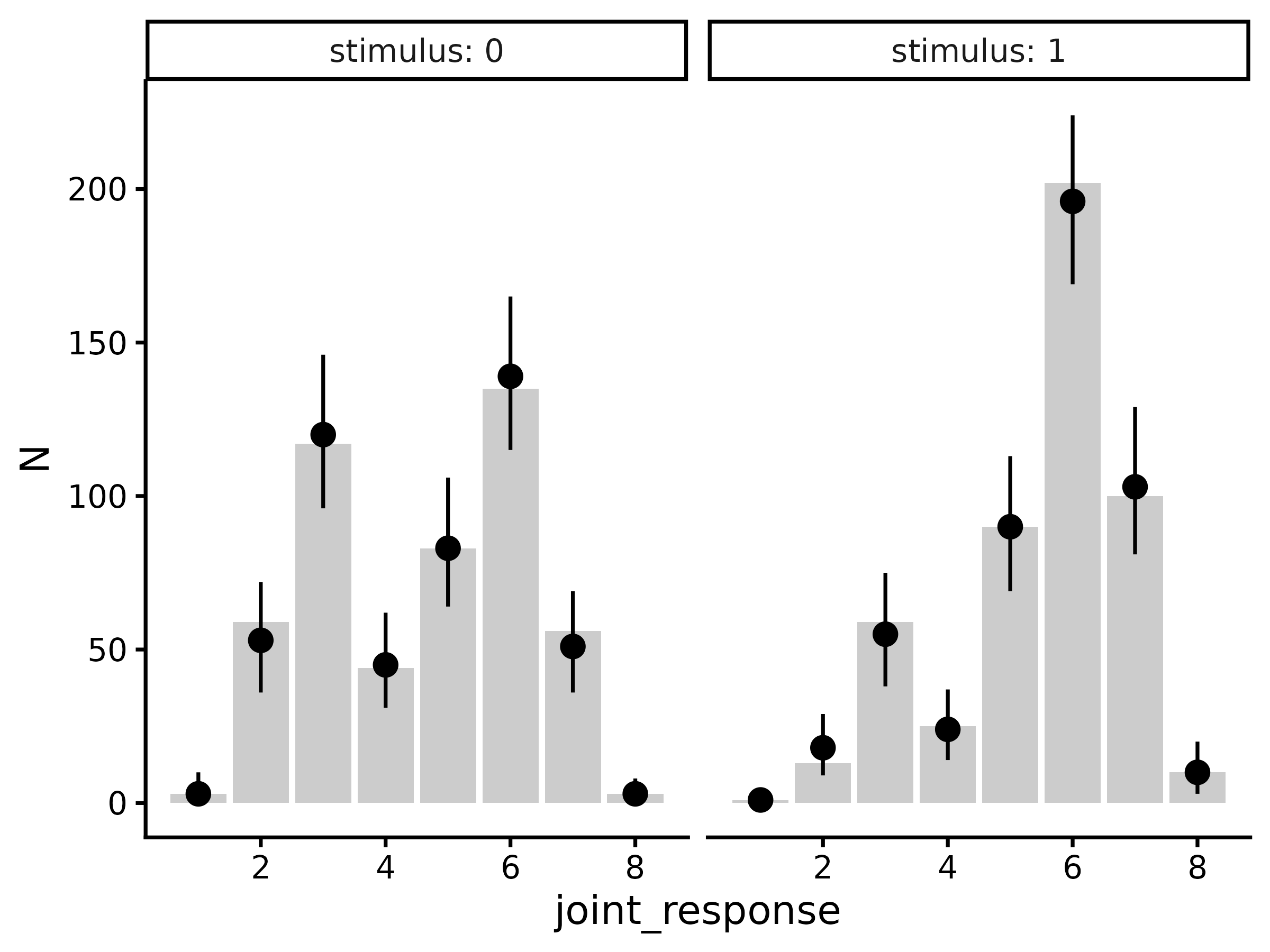
Posterior expectations
Usually it will be simpler to compare response probabilities rather
than raw response counts. To do this, we can use the same workflow as
above but using epred_draws_metad (which is a wrapper
around tidybayes::epred_draws):
draws.epred <- epred_draws_metad(m, newdata = tibble(.row = 1))#> # A tibble: 64,000 × 9
#> # Groups: .row, stimulus, joint_response, response, confidence [16]
#> .row stimulus joint_response response confidence .epred .chain .iteration
#> <int> <int> <int> <int> <dbl> <dbl> <int> <int>
#> 1 1 0 1 0 4 0.00329 NA NA
#> 2 1 0 1 0 4 0.00971 NA NA
#> 3 1 0 1 0 4 0.00485 NA NA
#> 4 1 0 1 0 4 0.00778 NA NA
#> 5 1 0 1 0 4 0.00277 NA NA
#> 6 1 0 1 0 4 0.00782 NA NA
#> 7 1 0 1 0 4 0.00646 NA NA
#> 8 1 0 1 0 4 0.00559 NA NA
#> 9 1 0 1 0 4 0.00789 NA NA
#> 10 1 0 1 0 4 0.00446 NA NA
#> # ℹ 63,990 more rows
#> # ℹ 1 more variable: .draw <int>
draws.epred |>
  group_by(.row, stimulus, joint_response, response, confidence) |>
  median_qi(.epred) |>
  group_by(.row) |>
  mutate(.true = t(response_probabilities(d.summary$N[.row, ]))) |>
  ggplot(aes(x = joint_response)) +
  geom_col(aes(y = .true), fill = "grey80") +
  geom_pointrange(aes(y = .epred, ymin = .lower, ymax = .upper)) +
  facet_wrap(~stimulus, labeller = label_both) +
  theme_classic(18)
#> Warning in `[<-.data.frame`(`*tmp*`, , y_vars, value = list(y = c(0.006, :
#> replacement element 1 has 256 rows to replace 16 rows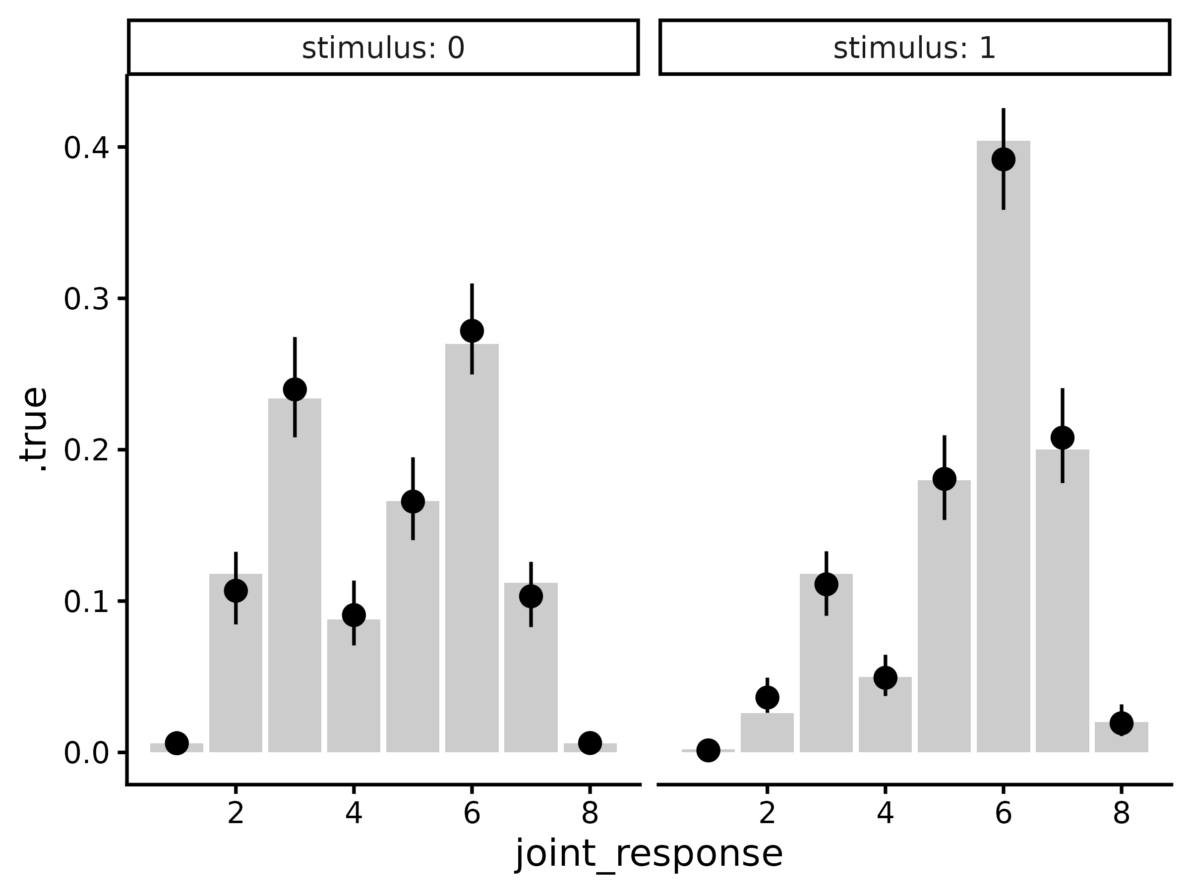
Mean confidence
One can also compute implied values of mean confidence from the
meta-d’ model using mean_confidence_draws:
tibble(.row = 1) |>
  add_mean_confidence_draws(m) |>
  median_qi(.epred) |>
  left_join(d |>
    group_by(stimulus, response) |>
    summarize(.true = mean(confidence)))
#> `summarise()` has regrouped the output.
#> Joining with `by = join_by(stimulus, response)`
#> ℹ Summaries were computed grouped by stimulus and response.
#> ℹ Output is grouped by stimulus.
#> ℹ Use `summarise(.groups = "drop_last")` to silence this message.
#> ℹ Use `summarise(.by = c(stimulus, response))` for per-operation grouping
#>   (`?dplyr::dplyr_by`) instead.
#> # A tibble: 4 × 10
#>    .row stimulus response .epred .lower .upper .width .point .interval .true
#>   <int>    <int>    <int>  <dbl>  <dbl>  <dbl>  <dbl> <chr>  <chr>     <dbl>
#> 1     1        0        0   2.07   1.99   2.15   0.95 median qi         2.09
#> 2     1        0        1   1.91   1.83   1.99   0.95 median qi         1.92
#> 3     1        1        0   1.95   1.86   2.03   0.95 median qi         1.90
#> 4     1        1        1   2.08   2.02   2.16   0.95 median qi         2.07
Here, .epred refers to the model-estimated mean
confidence per stimulus and response, and .true is the
empirical mean confidence.
In addition, we can compute mean confidence marginalizing over stimuli:
tibble(.row = 1) |>
  add_mean_confidence_draws(m, by_stimulus = FALSE) |>
  median_qi(.epred) |>
  left_join(d |>
    group_by(response) |>
    summarize(.true = mean(confidence)))
#> Joining with `by = join_by(response)`
#> # A tibble: 2 × 9
#>    .row response .epred .lower .upper .width .point .interval .true
#>   <int>    <int>  <dbl>  <dbl>  <dbl>  <dbl> <chr>  <chr>     <dbl>
#> 1     1        0   2.03   1.95   2.11   0.95 median qi         2.03
#> 2     1        1   2.01   1.96   2.07   0.95 median qi         2.01
over responses:
tibble(.row = 1) |>
  add_mean_confidence_draws(m, by_response = FALSE) |>
  median_qi(.epred) |>
  left_join(d |>
    group_by(stimulus) |>
    summarize(.true = mean(confidence)))
#> Joining with `by = join_by(stimulus)`
#> # A tibble: 2 × 9
#>    .row stimulus .epred .lower .upper .width .point .interval .true
#>   <int>    <int>  <dbl>  <dbl>  <dbl>  <dbl> <chr>  <chr>     <dbl>
#> 1     1        0   1.98   1.93   2.03   0.95 median qi         2
#> 2     1        1   2.06   2.01   2.11   0.95 median qi         2.04
or both over stimuli and responses:
tibble(.row = 1) |>
  add_mean_confidence_draws(m, by_stimulus = FALSE, by_response = FALSE) |>
  median_qi(.epred) |>
  bind_cols(d |>
    ungroup() |>
    summarize(.true = mean(confidence)))
#> # A tibble: 1 × 8
#>    .row .epred .lower .upper .width .point .interval .true
#>   <int>  <dbl>  <dbl>  <dbl>  <dbl> <chr>  <chr>     <dbl>
#> 1     1   2.02   1.97   2.06   0.95 median qi         2.02
Metacognitive bias
While mean confidence is often empirically informative, it is not recommended as a measure of metacognitive bias because it is known to be confounded by type 1 response characteristics (i.e., d' and c) and by metacognitive sensitivity (i.e., \textrm{meta-}d', Sherman et al., 2018). Instead, we recommend a new measure of metacognitive bias, \textrm{meta-}\Delta, which is the distance between the average of the confidence criteria and \textrm{meta-}c.
\textrm{meta-}\Delta can be interpreted as lying between two extremes: when \textrm{meta-}\Delta = 0, the observer only uses the highest confidence rating, and when \textrm{meta-}\Delta = \infty, the observer only uses the lowest confidence rating.
To obtain estimates of \textrm{meta-}\Delta, one can use the
function metacognitive_bias_draws:
tibble(.row = 1) |>
  add_metacognitive_bias_draws(m) |>
  median_qi()
#> # A tibble: 2 × 8
#>    .row response metacognitive_bias .lower .upper .width .point .interval
#>   <int>    <int>              <dbl>  <dbl>  <dbl>  <dbl> <chr>  <chr>
#> 1     1        0               1.15   1.02   1.29   0.95 median qi
#> 2     1        1               1.57   1.46   1.67   0.95 median qi
Pseudo Type 1 ROC
To obtain type 1 performance as a pseudo-type 1 ROC, we can use
add_roc1_draws:
draws.roc1 <- tibble(.row = 1) |>
  add_roc1_draws(m)
#> # A tibble: 28,000 × 9
#> # Groups: .row, joint_response, response, confidence [7]
#> .row joint_response response confidence .chain .iteration .draw p_fa p_hit
#> <int> <int> <int> <dbl> <int> <int> <int> <dbl> <dbl>
#> 1 1 1 0 4 NA NA 1 0.997 0.999
#> 2 1 1 0 4 NA NA 2 0.990 0.998
#> 3 1 1 0 4 NA NA 3 0.995 0.999
#> 4 1 1 0 4 NA NA 4 0.992 0.998
#> 5 1 1 0 4 NA NA 5 0.997 0.999
#> 6 1 1 0 4 NA NA 6 0.992 0.998
#> 7 1 1 0 4 NA NA 7 0.994 0.999
#> 8 1 1 0 4 NA NA 8 0.994 0.999
#> 9 1 1 0 4 NA NA 9 0.992 0.999
#> 10 1 1 0 4 NA NA 10 0.996 0.998
#> # ℹ 27,990 more rowsAgain, we have a tidy tibble with columns .chain,
.iteration, and .draw identifying individual
posterior samples, joint_response, response,
and confidence identifying the different points on the ROC,
and .row identifying different ROCs (since our data frame
has only one row, here there is only one ROC). In addition, we also have
p_hit and p_fa, which contain posterior
estimates of type 1 hit rate (i.e., the probability of a
"1" response with confidence >= c given
stimulus==1) and type 1 false alarm rate (i.e., the
probability of a "1" response with
confidence >= c given stimulus==0).
For visualization, we can get posterior summaries of the ROC using
tidybayes::median_qi and then simply plot as a line:
draws.roc1 |>
  median_qi(p_fa, p_hit) |>
  ggplot(aes(
    x = p_fa, xmin = p_fa.lower, xmax = p_fa.upper,
    y = p_hit, ymin = p_hit.lower, ymax = p_hit.upper
  )) +
  geom_abline(slope = 1, intercept = 0, linetype = "dashed") +
  geom_errorbar(orientation = "y", width = .01) +
  geom_errorbar(orientation = "x", width = .01) +
  geom_line() +
  coord_fixed(xlim = 0:1, ylim = 0:1, expand = FALSE) +
  xlab("P(False Alarm)") +
  ylab("P(Hit)") +
  theme_bw(18)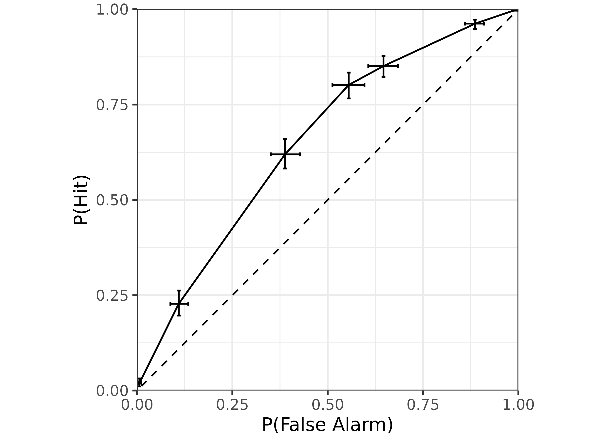
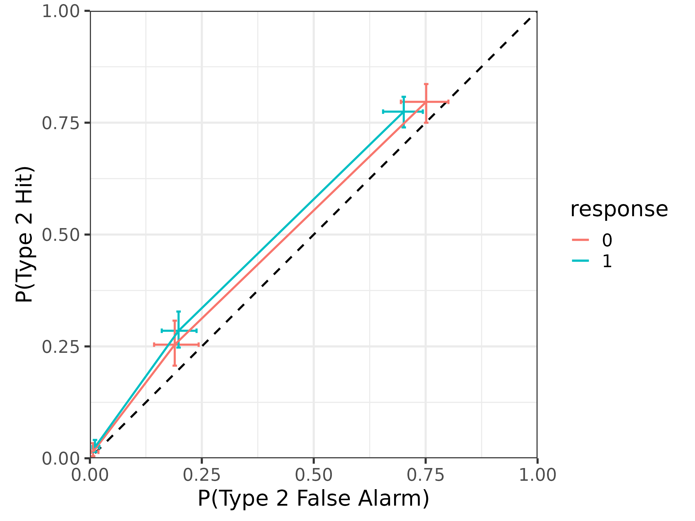
Type 2 ROC
Finally, to plot type 2 performance as a type 2 ROC, we can use
add_roc2_draws:
draws.roc2 <- tibble(.row = 1) |>
  add_roc2_draws(m)
#> # A tibble: 24,000 × 8
#> # Groups: .row, response, confidence [6]
#> .row response confidence .chain .iteration .draw p_hit2 p_fa2
#> <int> <int> <dbl> <int> <int> <int> <dbl> <dbl>
#> 1 1 0 4 NA NA 1 0.00722 0.00345
#> 2 1 0 4 NA NA 2 0.0236 0.0117
#> 3 1 0 4 NA NA 3 0.0103 0.00514
#> 4 1 0 4 NA NA 4 0.0174 0.00827
#> 5 1 0 4 NA NA 5 0.00670 0.00322
#> 6 1 0 4 NA NA 6 0.0185 0.00845
#> 7 1 0 4 NA NA 7 0.0148 0.00631
#> 8 1 0 4 NA NA 8 0.0126 0.00503
#> 9 1 0 4 NA NA 9 0.0162 0.00647
#> 10 1 0 4 NA NA 10 0.0114 0.00947
#> # ℹ 23,990 more rowsThis tibble looks the same as for roc1_draws, except now
there are columns for p_hit2 representing the type 2 hit
rate (i.e., the probability of a correct response with
confidence >= c given response) and the
type 2 false alarm rate (i.e., the probability of an incorrect response
with confidence >= c given response). Note
that this is the response-specific type 2 ROC, so there are two separate
curves for the two type 1 responses.
We can also plot the type 2 ROC similarly:
draws.roc2 |>
  median_qi(p_hit2, p_fa2) |>
  mutate(response = factor(response)) |>
  ggplot(aes(
    x = p_fa2, xmin = p_fa2.lower, xmax = p_fa2.upper,
    y = p_hit2, ymin = p_hit2.lower, ymax = p_hit2.upper,
    color = response
  )) +
  geom_abline(slope = 1, intercept = 0, linetype = "dashed") +
  geom_errorbar(orientation = "y", width = .01) +
  geom_errorbar(orientation = "x", width = .01) +
  geom_line() +
  coord_fixed(xlim = 0:1, ylim = 0:1, expand = FALSE) +
  xlab("P(Type 2 False Alarm)") +
  ylab("P(Type 2 Hit)") +
  theme_bw(18)