Using alternative signal distributions with the meta-d' model

Introduction

The standard meta-d’ model assumes that the evidence for making type 1 decisions follows an equal-variance normal distribution and that the evidence for making type 2 decisions follows a truncated equal-variance normal distribution. However, there has been recent interest in using other distributions in signal detection theory. While not all distributions will be identifiable with the meta-d’ model (e.g., one cannot simultaneously estimate unequal variances and \textrm{meta-}d'), the hmetad package allows one to specify any distribution that takes a single parameter defining the location (i.e., mean, median, or mode) of the distribution.

To demonstrate this functionality, here we implement the meta-d’ model with the Gumbel-min distribution, which has been shown to provide a parsimonious explanation of recognition memory data (Meyer-Grant et al, 2025).

We begin by loading necessary packages in R:

library(tidyverse)
library(brms)
library(tidybayes)
library(hmetad)

Implementing a distribution function for use with hmetad

In order for a distribution to be used with the hmetad package, one needs to implement its cumulative distribution functions in both R and Stan. Specifically, since the hmetad package computes the model likelihood on the logarithmic scale, one must define:

• <distribution>_lcdf(x, mu): the log cumulative distribution function defining \textrm{log } P(X \le x) for a random variable X \sim \textrm{distribution}(\mu).
• <distribution>_lccdf(x, mu): the log complementary cumulative distribution function defining \textrm{log } P(X \ge x) for a random variable X \sim \textrm{distribution}(\mu).

Please note that for use with the hmetad package, these two functions must use the above naming scheme (i.e., must be named <distribution>_l(c)cdf).

For example, we can write the gumbel min distribution functions in R as follows:

gumbel_min_lcdf <- function(x, g) {
  log1p(-exp(-exp(x - g)))
}
gumbel_min_lccdf <- function(x, g) {
  -exp(x - g)
}

One also needs to implement the two functions in Stan using brms::stanvar so that they are available to brms during model fitting. Fortunately, the functions themselves will usually look almost identical to their definitions in R, with only minor syntactic changes and/or use of more efficient helper functions. The code below implements the same two functions in Stan:

gumbel_min <- stanvar(
  scode = "
real gumbel_min_lcdf(real x, real g) {
  return log1m_exp(-exp(x - g));
}
real gumbel_min_lccdf(real x, real g) {
  return -exp(x - g);
}",
  block = "functions"
)

Again, note that the name of the functions in Stan must match their corresponding names in R. With the lcdf and lccdf functions implemented in both R and Stan, the new distribution is ready to use with the hmetad package!

Data simulation

Before continuing on to model fitting, this section describes how to simulate data from the meta-d’ model with your custom distribution. This is a necessary step for parameter recovery to ensure that the meta-d’ model is well-defined with respect to your distribution.

To simulate data, you can call the sim_metad function supplying the optional arguments lcdf and lccdf:

d <- sim_metad(
  N_trials = 10000, dprime = 1.5, c = .1, log_M = -.5,
  c2_0_diff = c(.25, .5, .25), c2_1_diff = c(.1, .5, .25),
  lcdf = gumbel_min_lcdf, lccdf = gumbel_min_lccdf
)

Model fitting

Once you have some data, fitting the model is exactly the same as with the equal-variance normal distribution, only now we also need to specify two additional arguments to fit_metad.

1. The distribution argument should be the name of the distribution as a string. This should be the part of the function names preceding "_lcdf" and "_lccdf" in both R and in Stan.
2. The stanvars argument should be the stanvar object you have created above containing the Stan code for your cumulative distribution functions.

Otherwise, one can call fit_metad just as with the equal-variance normal distribution! Please note, however, that the scale of all parameters will vary from distribution to distribution, so set priors accordingly. The code below shows how to fit the meta-d’ model with our new gumbel_min distribution:

m <- fit_metad(N ~ 1,
  data = d,
  prior = prior(normal(0, 1), class = Intercept) +
    prior(normal(0, 1), class = dprime) +
    prior(normal(0, 1), class = c) +
    prior(lognormal(-1, 1), class = metac2zero1diff) +
    prior(lognormal(-1, 1), class = metac2zero2diff) +
    prior(lognormal(-1, 1), class = metac2zero3diff) +
    prior(lognormal(-1, 1), class = metac2one1diff) +
    prior(lognormal(-1, 1), class = metac2one2diff) +
    prior(lognormal(-1, 1), class = metac2one3diff),
  distribution = "gumbel_min", stanvars = gumbel_min, file = "models/gumbel.rds"
)

#>  Family: metad__4__gumbel_min__absolute__multinomial 
#>   Links: mu = log 
#> Formula: N ~ 1 
#>    Data: data.aggregated (Number of observations: 1) 
#>   Draws: 4 chains, each with iter = 2000; warmup = 1000; thin = 1;
#>          total post-warmup draws = 4000
#> 
#> Regression Coefficients:
#>           Estimate Est.Error l-95% CI u-95% CI Rhat Bulk_ESS Tail_ESS
#> Intercept    -0.61      0.06    -0.73    -0.49 1.00     3591     3343
#> 
#> Further Distributional Parameters:
#>                 Estimate Est.Error l-95% CI u-95% CI Rhat Bulk_ESS Tail_ESS
#> dprime              1.55      0.03     1.49     1.61 1.00     5722     3474
#> c                   0.11      0.01     0.08     0.14 1.00     3812     2821
#> metac2zero1diff     0.24      0.01     0.22     0.26 1.00     5298     3297
#> metac2zero2diff     0.49      0.01     0.46     0.51 1.00     5293     3210
#> metac2zero3diff     0.25      0.01     0.23     0.27 1.00     6152     2811
#> metac2one1diff      0.10      0.01     0.09     0.11 1.00     4581     2940
#> metac2one2diff      0.48      0.01     0.45     0.50 1.00     4205     3027
#> metac2one3diff      0.25      0.01     0.23     0.27 1.00     4670     2731
#> 
#> Draws were sampled using sampling(NUTS). For each parameter, Bulk_ESS
#> and Tail_ESS are effective sample size measures, and Rhat is the potential
#> scale reduction factor on split chains (at convergence, Rhat = 1).

The model summary can be interpreted just as with any other model, however here you can see that the model family is metad__4__gumbel_min__absolute__multinomial, indicating that this model indeed uses the gumbel_min distribution with four confidence levels and \textrm{meta-}c = c.

Model estimates

Once the model is fit, it can be post-processed like any other model from the hmetad package. Because alternative distributions are often understood in terms of their effects on the ROC, here we will focus on plotting them.

Looking at the pseudo-type 1 ROC, we can see that the gumbel_min distribution exhibits an asymmetry:

# psuedo type-1 ROC
tibble(.row = 1) |>
  add_roc1_draws(m, bounds = TRUE) |>
  median_qi(p_fa, p_hit) |>
  ggplot(aes(
    x = p_fa, xmin = p_fa.lower, xmax = p_fa.upper,
    y = p_hit, ymin = p_hit.lower, ymax = p_hit.upper
  )) +
  geom_abline(slope = 1, intercept = 0, linetype = "dashed") +
  geom_errorbar(orientation = "y", width = .01) +
  geom_errorbar(orientation = "x", width = .01) +
  geom_point() +
  geom_line() +
  coord_fixed(xlim = 0:1, ylim = 0:1, expand = FALSE) +
  xlab("P(False Alarm)") +
  ylab("P(Hit)") +
  theme_bw(18)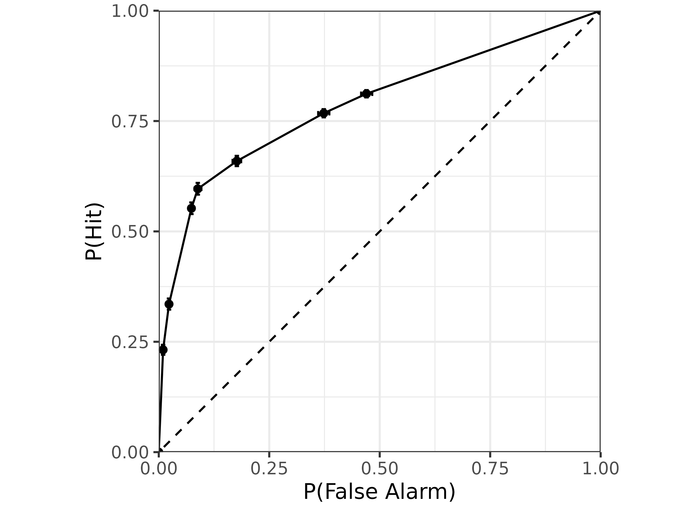

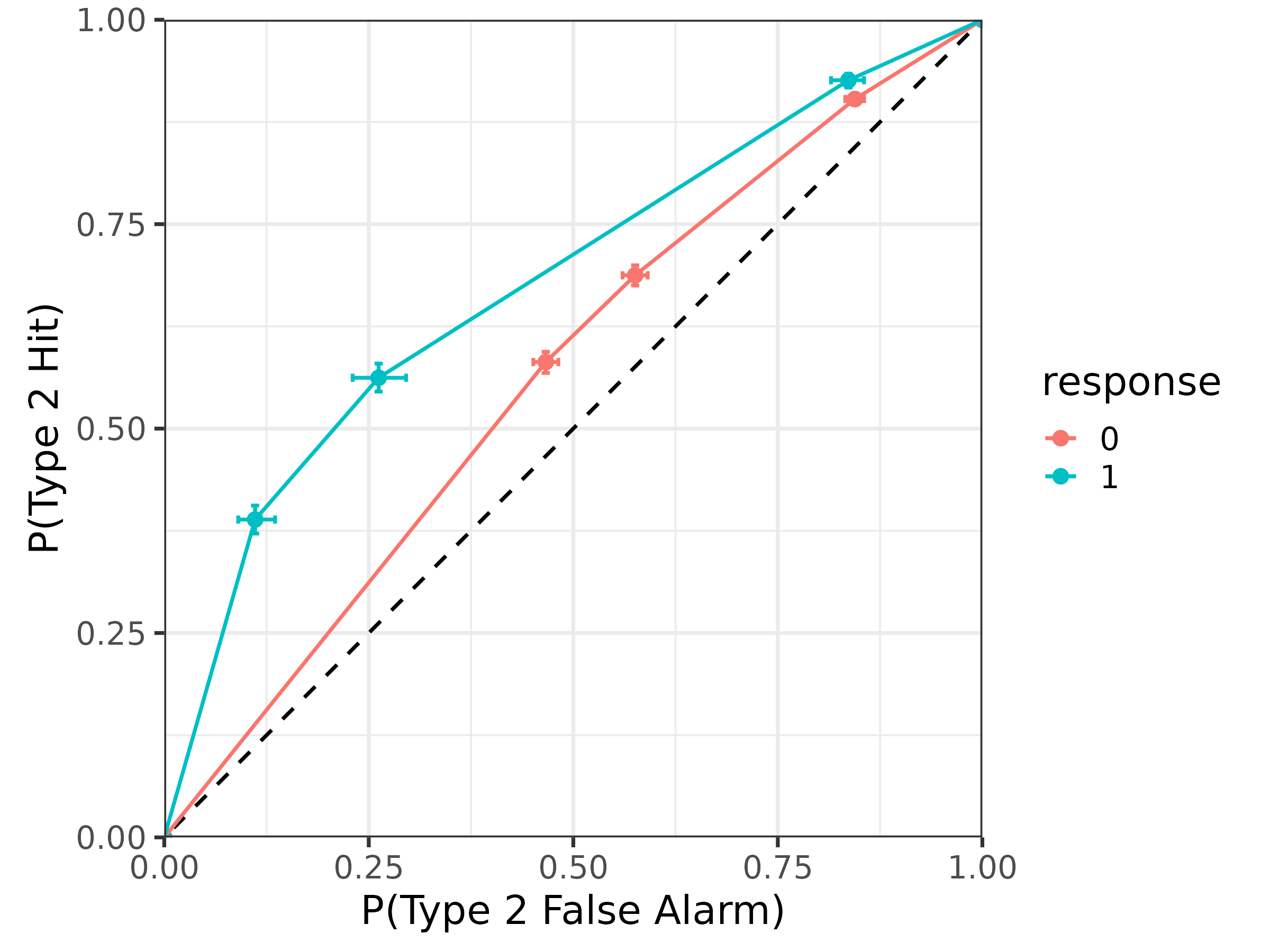
Likewise, the gumbel_min distribution also has asymmetric type 2 ROCs:

# type 2 ROC
roc2_draws(m, tibble(.row = 1), bounds = TRUE) |>
  median_qi(p_hit2, p_fa2) |>
  mutate(response = factor(response)) |>
  ggplot(aes(
    x = p_fa2, xmin = p_fa2.lower, xmax = p_fa2.upper,
    y = p_hit2, ymin = p_hit2.lower, ymax = p_hit2.upper,
    color = response
  )) +
  geom_abline(slope = 1, intercept = 0, linetype = "dashed") +
  geom_errorbar(orientation = "y", width = .01) +
  geom_errorbar(orientation = "x", width = .01) +
  geom_point() +
  geom_line() +
  coord_fixed(xlim = 0:1, ylim = 0:1, expand = FALSE) +
  xlab("P(Type 2 False Alarm)") +
  ylab("P(Type 2 Hit)") +
  theme_bw(18)